Ginzburg–Landau

The real Ginzburg–Landau system in 2D, written for the pair $(u,v)$ — spiral waves emerge from the reaction terms:

$$\frac{\partial u}{\partial t}=\epsilon {\mathrm{\nabla }}^{2}u+k[u-(u^2+v^2)u-1.5(u^2+v^2)v],$$$$\frac{\partial v}{\partial t}=\epsilon {\mathrm{\nabla }}^{2}v+k[v-(u^2+v^2)v+1.5(u^2+v^2)u].$$

Results

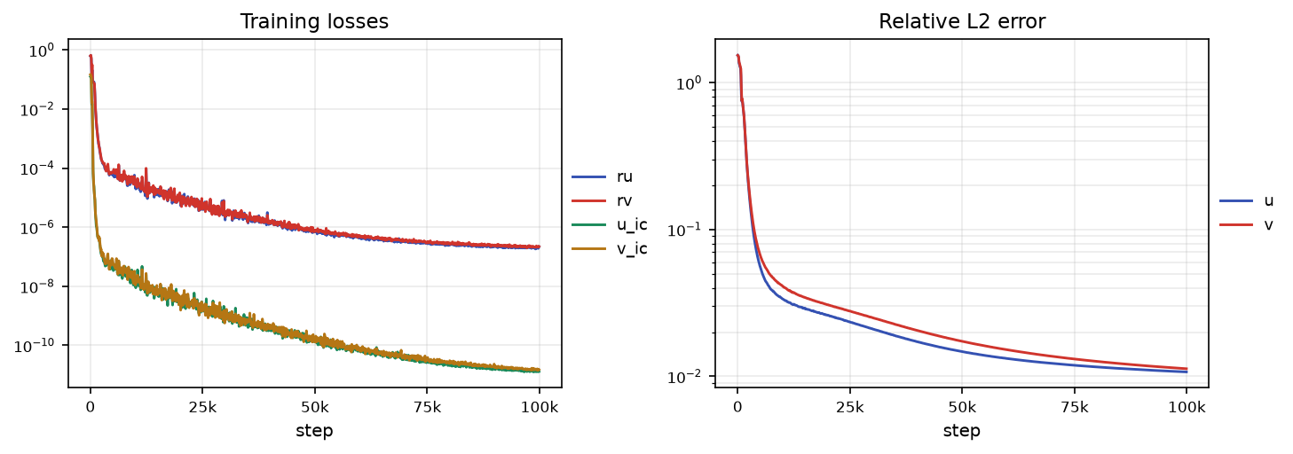
relative L2 error 0.011recipe adaptive pseudo-time100k steps, single GPU

The rotating spiral is captured to a relative L2 error of 0.011 with adaptive pseudo-time stepping — a 4× improvement over the baseline's 0.042. Ginzburg–Landau has the classic spurious-attractor structure (the homogeneous state is a residual minimizer), and the damping term is what keeps training locked onto the rotating solution as the wavefront sweeps the domain. The animation below shows the prediction tracking the reference through a full rotation; the error stays confined to the spiral arms where the field gradients are steepest.

Reference, PINN prediction, and absolute error of the u-field over time.

Training losses and per-variable relative L2 errors of the showcase run.

Run

cd examples/ginzburg_landau
python3 main.py --config=configs/pseudo_time.py

Config	Description
configs/baseline.py	PirateNet + causal weighting
configs/pseudo_time.py	Adaptive pseudo-time stepping (showcase)
configs/fixed_pseudo_time.py	Constant pseudo-time weights

Notes

• Time-window training with MeshSampler initial conditions: the IC data flows through the batch, so each window simply resamples from the propagated field.
• The two residuals are keyed by their variables (u, v) — see the variable-keyed residual convention.