Pseudo-Time Stepping

TL;DR

The empirical residual loss can be small on a spurious solution — sharp transition layers hide between collocation points. Pseudo-time stepping augments the residual with an implicit-Euler damping term toward the previous iterate, which (together with resampling) amplifies these hidden defects so the optimizer must fix them. Based on Wang, Koohy, Lu & Perdikaris, When PINNs Go Wrong, 2026.

The problem: spurious solutions with small losses

PINN training sometimes converges to physically wrong solutions despite tiny residual losses. The paper argues this is not an optimization failure but a defect of the empirical loss itself: profiles with a sharp transition layer of width $h$ concentrate their residual in a region a finite collocation set barely samples, so a spurious solution can look nearly perfect to the loss.

The fix: relax in pseudo-time

Introduce an artificial relaxation $\partial u/\partial s+\mathcal{R}[u]=0$ in pseudo-time $s$ and discretize implicitly with step $\tau$ (paper, Eqs. 2.37–2.39). At training step $k$, the residual loss becomes

$${\mathcal{L}}_{\mathrm{pts}}(\theta ;{\theta }^{k-1})=\frac{1}{N}\sum _{i=1}^N{|\frac{u_{\theta }(x_i)-u_{{\theta }^{k-1}}(x_i)}{\tau }+\mathcal{R}[u_{\theta }](x_i)|}^2,$$

i.e. the plain residual plus a damping term $\frac{1}{\tau }(u_{\theta }-u_{{\theta }^{k-1}})$ toward the previous iterate. Systems of PDEs get one step size per component (${\tau }_u,{\tau }_v,{\tau }_p,\dots$).

Why it works (the paper's key insight): one pseudo-time update $u^{†,+}=u^{†}-\tau \mathcal{R}[u^{†}]$ applied to a spurious profile amplifies the expected residual on freshly resampled collocation points from $O(h^{-1})$ to $O({\tau }^2{h}^{-3})$ — the hidden defect becomes glaring, and training is steered away from the spurious attractor. Collocation resampling is essential to the mechanism.

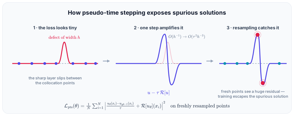
Adaptive step size

The amplification grows with $\tau$, but too large a $\tau$ makes the relaxed objective unstable — and the sweet spot cannot be read off the training loss. The paper's adaptive strategy picks the largest locally stable step from a Barzilai–Borwein-style finite-difference surrogate of the residual Jacobian. Per component, JAXPI computes

$$w=\frac{1}{\tau }=\frac{\Vert \mathcal{R}[u_{\theta }]-\mathcal{R}[u_{{\theta }^{prev}}]\Vert }{\Vert u_{\theta }-u_{{\theta }^{prev}}\Vert },$$

smoothed with momentum and clipped — a local estimate of the residual's Lipschitz constant. An optional cosine shrink schedule decays the weights as the true residual converges, so the damping vanishes near the solution.

In JAXPI

pseudo_time.enabled = True
pseudo_time.strategy = "dynamic"          # adaptive tau; "constant" for fixed weights
pseudo_time.pts_weights = {"u": 1.0, "v": 1.0, "p": 1.0}   # 1/tau per variable
pseudo_time.update_schedule = {"start": 100, "every": 1000}
pseudo_time.shrink.enabled = True

The residual components and their weights are matched by name — hence the variable-keyed residual convention.

Where it's used

Every example ships pseudo_time.py / fixed_pseudo_time.py config variants. The clearest demonstrations are Gray–Scott and Ginzburg–Landau (spurious steady states), inviscid Burgers (spurious weak solutions), and the high-Re lid-driven cavity.