PirateNets

TL;DR

Deep PINNs train worse than shallow ones because bad initialization of the network derivatives destabilizes the residual loss. PirateNets add a trainable skip $\alpha$ (initialized at 0) to every residual block, so the model starts as a linear map of its embeddings and deepens itself during training. Based on Wang, Li, Chen & Perdikaris, JMLR 2024.

The problem: depth hurts PINNs

For standard MLPs with common initializations, the derivatives of the network — which is what the PDE residual sees — become increasingly pathological with depth. Empirically, PINN accuracy degrades as MLPs get deeper, the opposite of what we expect from deep learning.

The architecture

Input coordinates are first lifted by an embedding $\mathrm{\Phi }(x)$ (random Fourier features in JAXPI), from which two gating states are computed once:

$$U=\sigma (W_u\mathrm{\Phi }(x)+b_u),V=\sigma (W_v\mathrm{\Phi }(x)+b_v).$$

Each residual block $l$ then applies three dense layers with two gating operations (paper, Eqs. 19–24):

$$\begin{array}{rlrl}{f}^{(l)}& =\sigma (W_1^{(l)}{x}^{(l)}+b_1^{(l)}),& z_1^{(l)}& =f^{(l)}\odot U+(1-f^{(l)})\odot V,\\ g^{(l)}& =\sigma (W_2^{(l)}{z}_1^{(l)}+b_2^{(l)}),& z_2^{(l)}& =g^{(l)}\odot U+(1-g^{(l)})\odot V,\\ h^{(l)}& =\sigma (W_3^{(l)}{z}_2^{(l)}+b_3^{(l)}),& x^{(l+1)}& ={\alpha }^{(l)}{h}^{(l)}+(1-{\alpha }^{(l)})x^{(l)}.\end{array}$$

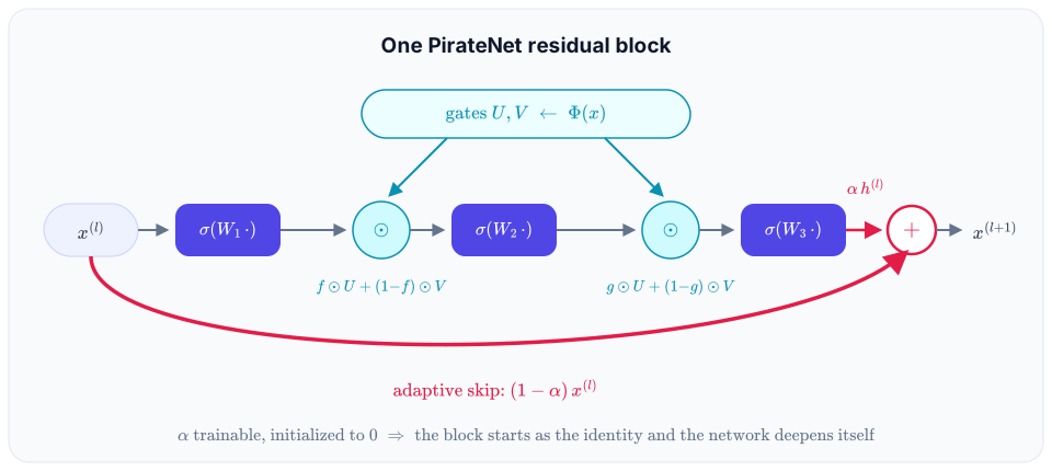
The key design is the adaptive skip ${\alpha }^{(l)}\in \mathbb{R}$:

• ${\alpha }^{(l)}=0$: the block is an identity map — the whole network reduces to a linear combination of the first-layer embeddings, which is trivially well-conditioned for the residual loss.
• ${\alpha }^{(l)}=1$: a fully nonlinear block with no shortcut.

Initializing ${\alpha }^{(l)}=0$ means the model starts shallow and deepens as training demands — the nonlinearities switch on only when they reduce the loss. A PirateNet with $L$ blocks has depth $3L$ but trains as robustly as a shallow network. The paper additionally proposes a physics-informed least-squares initialization of the final linear layer when data is available.

In JAXPI

arch.arch_name = "PirateNet"
arch.num_layers = 2                 # residual blocks (depth 3L)
arch.hidden_dim = 256
arch.nonlinearity = 0.0             # initial alpha for every block
arch.fourier_emb = {"embed_scale": 2.0, "embed_dim": 256}   # must equal hidden_dim

The learned ${\alpha }^{(l)}$ values can be logged during training (logging.log_nonlinearities = True) — watching them grow is a nice window into how much depth the problem actually needs.

Where it's used

The default architecture of nearly every benchmark; the Taylor–Green multi-stage cascade relies on it at every stage. See Architectures for the other options.